Mihai-Albert.com

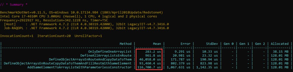
In the first part of this 3-article series, we’ve found to our astonishment that code based on ArrayList performs a whole lot worse than the same one using List<T>.

In order to understand why this is so, we’ll break up the code in smaller parts, see what these involve under the hood and how much time each takes. We should then be able to pinpoint the operation(s) that have the major contribution to the difference in performance. We’ll do this for both structures, and start with ArrayList in this post.

Before moving forward, please note that the discussion will be around the .NET Framework for Windows. All the code discussed is 32-bit (x86), although the concepts are applicable to x64 as well. Also all the benchmarked code is compiled in “Release” mode. In terms of GC, we’re specifically looking at Concurrent Workstation GC, not Server GC.

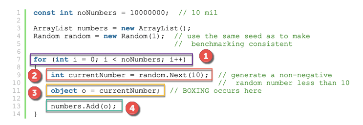
First, let’s take the initial code and slightly rewrite it, so the individual boxing operation is easily seen (full sample code here):

            const int noNumbers = 10000000;  // 10 mil

            ArrayList numbers = new ArrayList();
            Random random = new Random(1);  // use the same seed as to make
                                            //  benchmarking consistent

            for (int i = 0; i < noNumbers; i++)
            {    
                int currentNumber = random.Next(10);  // generate a non-negative
                                                      //  random number less than 10
                object o = currentNumber;  // BOXING occurs here

                numbers.Add(o);
            }

Let’s identify and highlight each operation:

In addition to the list above, there’s something else going on as well, namely Garbage Collection (GC). Let’s briefly discuss this next.

Garbage Collector

What is Garbage Collection? A definition below:

The managed memory occupied by unused objects must also be reclaimed at some point; this function is known as garbage collection and is performed by the CLR.

Joseph Albahari, Ben Albahari. C# 7.0 in a Nutshell: The Definitive Reference

An intro to this topic – including the managed heap, generational model, blocking/non-blocking collections, etc – is in this Microsoft article. Whole chapters and entire books have been written about the GC. One such book – which I’ve read extensively while working on this post – is Konrad Kokosa’s “Pro .NET Memory Management“. It goes very deep into the inner workings of the GC, and the time spent reading it is well invested. As such, only the GC topics that the investigation will directly depend on will be discussed when they’re required in the article.

Coming back to our investigation – we’ll want to know how much the GC spends as well, since the total time required to run the ArrayList sample will be the sum of the 4 highlighted sections above, plus the time spent doing GC.

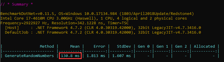
Do we have reasons to believe that GC affects either the ArrayList or the List<T> samples? For that we’d need to know if GC runs during either of the samples, and luckily BenchmarkDotNet can show GC activity right in the output:

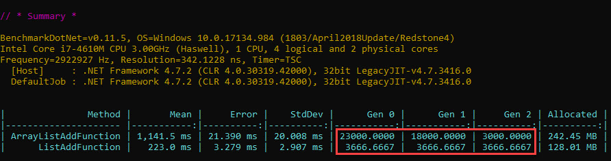
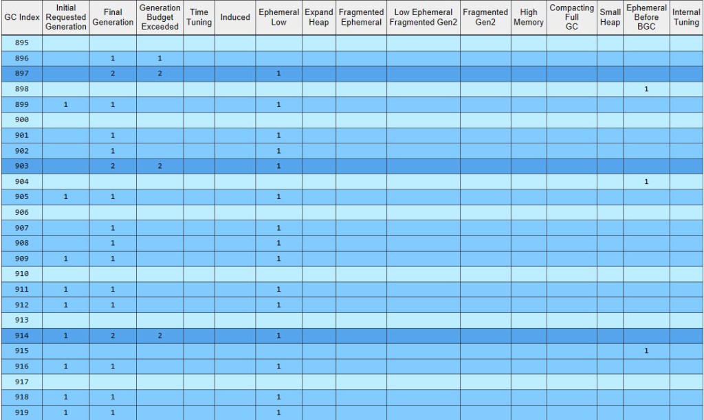
The numbers represent how many GCs per 1000 runs occur. So for one run of our ArrayList sample code, there are on average 23 gen0, 18 gen1 and 3 gen2 GCs.

In the upcoming analysis, we’ll need data about when exactly garbage collections (GCs) occur and how long they take. Aside BenchmarkDotNet, 2 more tools will be used to get detailed info about it: JetBrains’ dotTrace and PerfView. Both rely on ETW (Event Tracing for Windows) to get GC times, which will allow precise measurements to be made.

BenchmarkDotNet (BDN)

Since we need reliable time measurement for the various pieces of code we’ll test, BenchmarkDotNet will be employed quite heavily. Why not just use StopWatch to measure how long operations take? That’s pretty precise after all, right? Well, not quite. Unlike using BDN, you lose having automatic repeated iterations, warmup stages, loop unroll prevention, hardware platform’s overhead taken into account, outlier removal, etc. You can read about the topic of benchmarking from the author of BDN himself – Andrey Akinshin – in his excellent book “Pro .NET Benchmarking“. Due to the gotchas and insightful information within, I’ve read this one completely while working on this blog post, and would highly recommend it to anyone concerned with .NET performance measurement.

Our plan will be simple – use BDN to time each of the 4 operations we’ve identified above in isolation. Then we’ll sum this up and see if it matches the time it took our sample to run. If it does, then we’ll try to figure out why the part that takes so much does so; if however the sum for the 4 operations’ time doesn’t match the sample’s time, then we’d need to dig deeper and figure out if there’s a 5th operation or something else that has a bearing on our problem.

An important thing is that the code that will be benchmarked is indeed doing what we’d like it to do. The problem is this: when the code is first compiled, it gets translated to IL. Then when the code gets to execute, the IL is transformed by the CLR’s JIT compiler into native code. The problem is that sometimes the C# code that we write doesn’t translate into the desired native code eventually. One example is dead code elimination (DCE), where the compiler will simply leave out instructions that it determines have no effect (eg computing values that are not used subsequently). Another example is loop unrolling, whereby a for loop whose loop variable is incremented by 1 in the C# code gets translated under the right conditions in machine code that increments by 4 and counts up to N/4. In both cases the time measured will be smaller than the one we are searching for; even more still, the result in the first example won’t even be remotely correct.

Seeing the actual machine code will set the expectations right, and luckily BDN can extract the assembly instructions for us by simply using the DisassemblyDiagnoser attribute.

Since the GC can kick in and greatly increase the time taken for a particular benchmark, care must be taken so that we don’t inadvertently trigger it. After all, we want to measure how long boxing 10 mil elements took, not the time required for their boxing and the time GC “stole” as well.

For some of our operations – this won’t be a problem. In our example, generating the random numbers just involves calling a method and storing the result in same variable on the stack. Nothing is allocated directly on the heap, so GC won’t kick in and the measured time for this benchmark will only reflect what we’re after. For boxing however, it’s not so simple. Allocating the 10 mil objects on the heap will trigger the GC repeatedly, which in turn will result in our main managed thread being blocked, which will translate in inflated measured time for the benchmark.

So how much GC can be accepted in order for the results to be meaningful? Would one GC only per iteration be a cause for concern or would one GC in fact be one too many? Suffice to say at this stage that should just one GC intervene while a BDN benchmark is running, there are specific scenarios where one can see simple operations, which are quick in themselves and taking several hundred milliseconds, end up – due to a high GC time that gets averaged out – being measured at 10 times their real time. Stating a measured time of 4 ms instead of 400 us and factoring this in further computations would produce the wrong conclusions*. So we either strive not to have any GC occurring, or allow GCs only if we’re able to measure their exact time and subtract it afterwards. Both ways will get us the effective time, and both will be employed in this article.

As to how a BDN benchmark unfolds for a specific method: its code is run for a specific number of times – called operations (ops) – in sequence. The code is run essentially back-to-back, meaning there’s no pause between the operations. One such sequence of operations is called an iteration. There’s also a number of iterations ran. Between 2 subsequent iterations, the GC is manually invoked by BDN, and will show up as 4x gen2 non-concurrent GCs to the tools analyzing GC activity. So one operation is the method’s code running just once, one iteration is a number of operations ran one after the other, and the whole run is a number of iterations. This workflow is captured in BDN’s documentation here.

To conclude, individual BenchmarkDotNet projects will be created for each of the 4 parts seen in figure 1 – namely (1) the loop, (2) generating the random numbers, (3) boxing the values and (4) adding the elements to the ArrayList – in order to measure the time each takes.

Assembly Code

In order to make sure the total (the ArrayList sample code) is indeed the sum of all its constituent parts that will be benchmarked in isolation – we’ll have to look at the resulting assembly code for each and ensure that when they’re put together they match our ArrayList sample.

Let’s look first at the loop for the ArrayList sample’s assembly code, as it’s resolved by BenchmarkDotNet, and delimit each operation using the color code we’ve employed previously in figure 1:

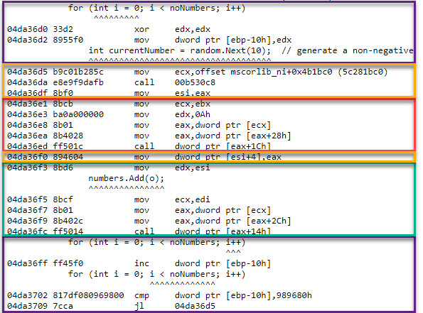
The hex addresses to the left is where in the virtual memory the respective native (machine) instruction was placed at. Next come the bytes that codify the instruction’s opcode and operands (data), followed by its human-readable version. Interspersed throughout the assembly lines is the corresponding C# code.

Let’s discuss each of the operations in turn.

The Loop

Since a loop is used to add the elements to the ArrayList sample as well as the List<T> one, it’s obvious that this isn’t the culprit in our performance difference. The for instruction itself – that is 1 x [initialising the loop counter variable], 10m x [loop counter increment] and 10m x [comparing the loop counter against the 10 mil value] – all things being equal – should take the same amount of time in both cases.

To find out how long is spent in the loop instructions, the easiest way would be to just write a simple BDN benchmark with only one method which consists of just a loop. The compiler however can implement this in 2 ways:

• Optimized: one register – as in eax / ebx / etc – is used to store the loop counter value, provided there’s one available
• Non-optimized: stack locations are used – eg ebp-<offset> – for the loop counter value

If you look back at figure 3 over the full sample’s loop code, you can see that a stack location (ebp-10h) is used. But does it really matter for us which version is chosen by the compiler?

Let’s write a BDN benchmark with 2 loop methods, one non-optimized and the other optimized (full code here) and see the results:

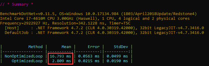
That’s quite a difference, albeit not much in absolute terms. Let’s look at the assembly code – below we have both methods side-by-side, as produced by BDN:

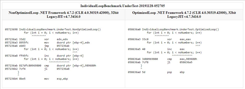
Both methods do the same thing: either a location on the stack (ebp-4; left, non-optimized method) or a register (eax; right, optimized method) is used to store the value of the loop counter. It’s first set to 0 – by performing an xor against itself, then within the loop its value is incremented (inc) and checked (cmp) against the limit (989680h, the hex representation of 10 mil).

So why do we care about this whole optimized/non-optimized business? Well, the BDN samples are all compiled to Release mode – this being a default requirement of BDN – which results in optimized code to be generated when possible. The catch is that parts of the code can’t always be optimized – specifically for our for instruction, sometimes the JIT cannot generate an implementation based on a cpu register. It’s actually the case with the full sample in figure 3. The cause of this “failure to optimize” is beyond us, the bottom line is that the JIT opted for a stack-backed value, despite us instructing it to compile in an optimized manner.

Yet we’ll be analyzing further parts of the code in isolation, and they’ll each involve a loop. As we’re about to see, for some of these the machine code implementation of the for instruction will be successfully optimized – that is it’ll use registers. And since we’re after the time of that respective operation only (excluding the time for the loop), we’d need to subtract the correct time value for the loop: either the one for the non-optimized loop (~17 ms), or the one for the optimized one (~3 ms). Since we’ll have access to the BDN disassembled code for all the parts we’ll be analyzing, based on where the loop counter value is stored (stack vs register) we’ll be able to subtract the right value.

Generating the Random Numbers

Just as discussed for the loop – it’s quite certain that generating the random numbers also isn’t the culprit for the performance degradation, given that this operation is performed in both cases as well.

The assembly code produced by the isolated BenchmarkDotNet project for generating the random numbers (C# full code here) is below. Note that only the loop where the random numbers are generated is shown; the initialization part is left out. The == comments have been added manually afterwards to make the code more clear.

            for (int i = 0; i < noNumbers; i++)
                 ^^^^^^^^^
058036b5 33ff            xor     edi,edi
                currentNumber = random.Next(10);  // generate a non-negative
                ^^^^^^^^^^^^^^^^^^^^^^^^^^^^^^^^
==Load the MethodTable's address for the Random type==
058036b7 8bce            mov     ecx,esi
==Prepares the parameter 10 (0A in hex) to be passed next==
058036b9 ba0a000000      mov     edx,0Ah
==Gets address of the Random.Next method==
058036be 8b01            mov     eax,dword ptr [ecx]
058036c0 8b4028          mov     eax,dword ptr [eax+28h]
==Calls Random.Next (result of the method will be stored in eax)==
058036c3 ff501c          call    dword ptr [eax+1Ch]
            for (int i = 0; i < noNumbers; i++)
                                           ^^^
058036c6 47              inc     edi
            for (int i = 0; i < noNumbers; i++)
                            ^^^^^^^^^^^^^
058036c7 81ff80969800    cmp     edi,989680h
058036cd 7ce8            jl      058036b7

The time that will be measured by BDN also includes the loop itself. The value below:

In the previous section we’ve already looked at the loop time, and , since it’s quite visible that this time a register (edi) is used for the loop counter, we can easily obtain the time spent just generating the random numbers. Subtracting the time for the optimized loop (3 ms) yields approximately 127 ms for generating the 10 mil random numbers.

Boxing

Next on the list is boxing. We do need to time this operation in isolation though, so we can’t go around boxing random numbers, since that will first mean generating the random numbers, and we’ve already measured that. Sure, the time for the random numbers could be subtracted afterwards, similar to the loop time, but let’s keep things simple. We can either box a constant number, or something that will already be “warm” – such as the loop counter variable.

Let’s look at the resulting source code for the method that will be timed (full source code here):

const int noNumbers = 10000000;  // 10 mil
 
object o = null;
for (int i = 0; i < noNumbers; i++)
{
     o = i;  
}
int v = (int)o;

Unlike the previous sections (the loop itself and generating the random numbers) there’s something else that will creep up this time – the Garbage Collector (GC). Since boxing involves allocating space on the heap, all that allocated memory becomes eligible for inspection by the GC. And because we don’t really hang on to the boxed objects – since our o variable always points to a new boxed int, essentially abandoning the previous one – the GC has work to do.

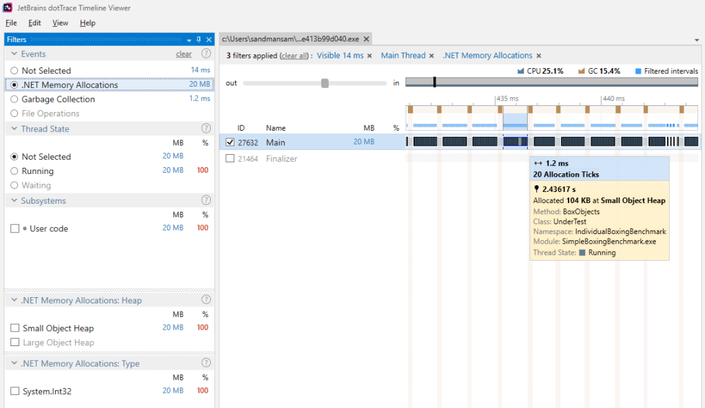
Since the int objects have the references towards them quickly “severed”, they won’t make it very far in the generational model. As such gen0 GCs will be responsible for collecting them. Here’s a view of how this looks like – each allocation tick represents the moment at least 100 KB worth of objects (roughly 8500 objects considering there are 12 bytes/boxed int) have been allocated on the heap. Note that after around 20 such allocations a gen0 GC kicks in. The pattern is repeated across the entire timeline for the 10 mil elements.

Knowing this, let’s look at the results BenchmarkDotNet produces for our boxing code. The last 2 iterations are highlighted:

Yet the time we’re after is the time taken to box the 10 mil int values, not the one including how much the GC spends while the boxing occurs.

PerfView can be used to extract the time spent doing GCs through the GCStats view, which captures the time it takes suspending the EE as well as for the GCs themselves. We just need to ensure that it’s already running before starting the BenchmarkDotNet code. We’ll also be using GC Collect only option, so that the overhead introduced by PerfView is minimal, and only info about GCs is collected. As for the BDN iterations, we’ll keep them low (10) so that PerfView’s output data isn’t huge.

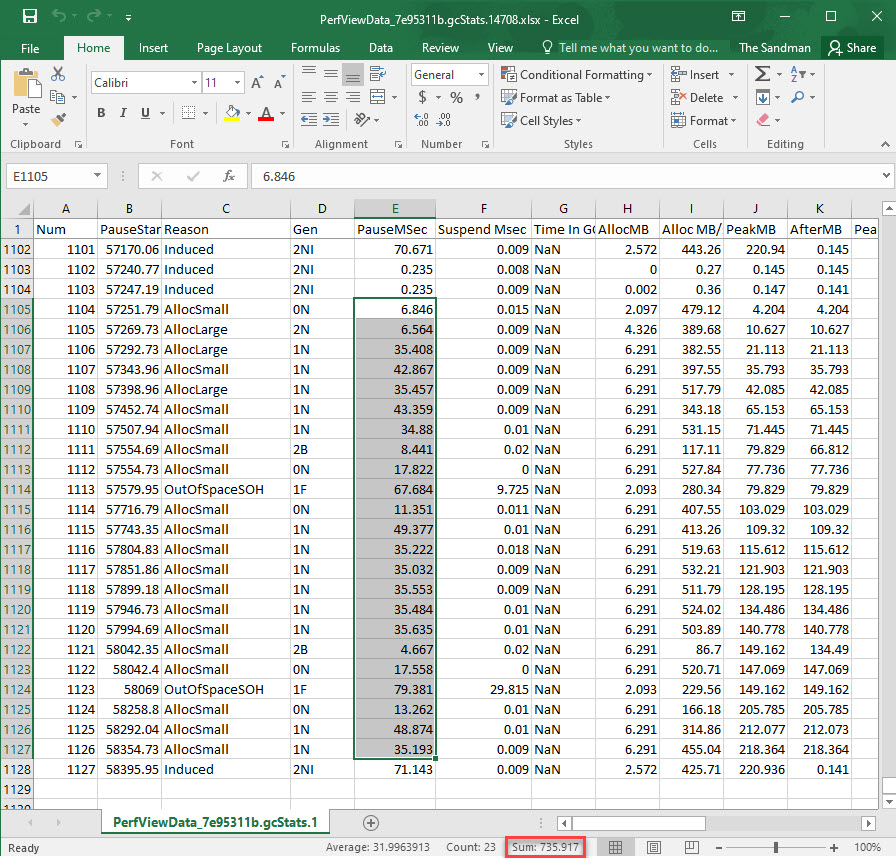
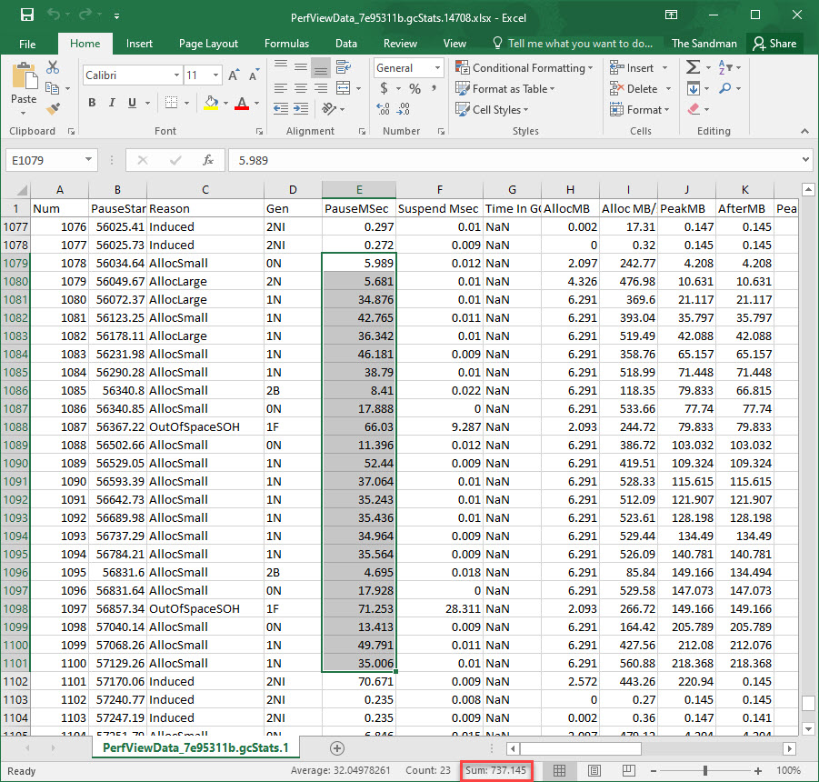
Once PerfView parses the data, it generates the GCStats view, based on which the time spent in GCs can be obtained per each iteration. Given that PerfView can export the GC results in an Excel file, and that we’re dealing only with gen0 GCs, which are blocking, it all comes down to summing up the values for the PauseMSec column, which will represent the time the gen0 GCs actually took, equivalent to the time the managed threads were suspended. As for the rows where the values will be summed up, we’re targeting those belonging to a specific iteration, which can be easily identified since after each iteration BenchmarkDotNet does induced GCs, which are clearly marked as such. Here’s part of the data for the GCs for the very last iteration from the 2 highlighted in the previous picture, and note the sum of the gen0 GC time for this iteration:

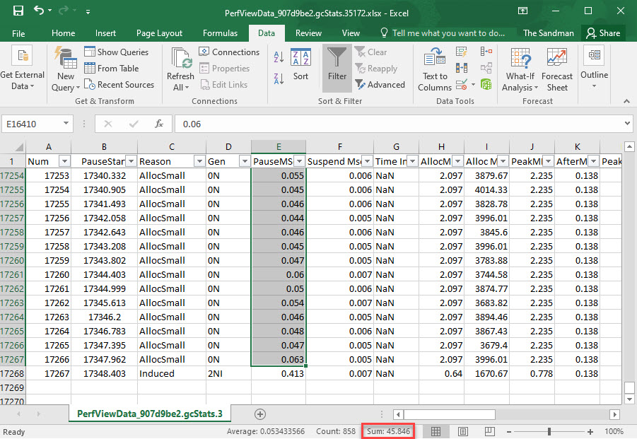
Finally we need to subtract the time computed for the gen0 GCs from the overall time that BenchmarkDotNet reports, and divide by the number of ops in order to arrive at the time spent for boxing our 10 mil int values. Take care to use the time for the whole iteration (value in ns in figure 8), not the average one computed per op (value in ms in figure 8) – since the “block” of GCs for which we summed the time was per the whole iteration, not per an op.

Summing for the penultimate iteration, we get 46.58 ms GC time, comparable with the GC time for the last iteration (computed before, 45.84 ms). Since there are 15 ops/iteration, that comes down to roughly 3.1 ms GC time per boxing 10 mil ints.

Let’s look at the final output for BenchmarkDotNet against our simple boxing code:

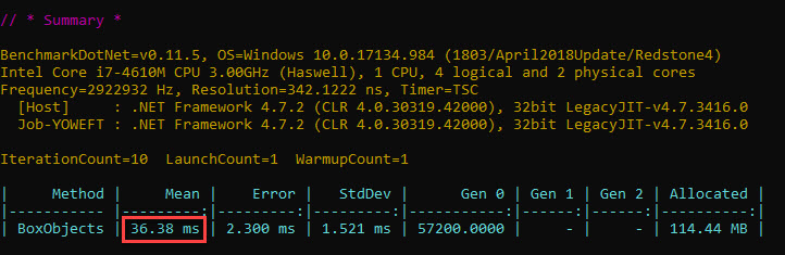
Subtracting the 3.1 ms GC time from above, and the time for the optimized loop (3 ms), the time for boxing 10 mil int values – not counting GC – is roughly 30 ms on this hardware platform.

Too Much of a Surprise?

Thinking of how incriminated boxing is for taking lots of time, the results above clearly surprise. After all, generating the random numbers took approximately 4 times as long (140.7 ms, as presented in the previous section). How come boxing is this fast?

As seen in the previous part of this article boxing consists of 3 phases: (a) allocating memory, (b) copying the source value and (c) returning a reference to the new object.

The description above is good on paper, but in C# the boxing instruction is reduced to one statement as we’ve seen. It’s the same thing in IL, where the box instruction is what we end up with. But in assembler, to which the IL eventually compiles to, things start to get more interesting.

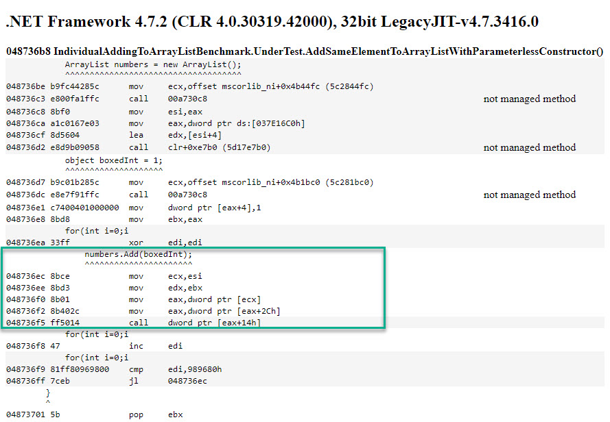
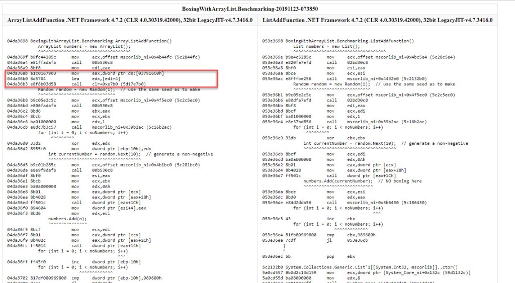
Let’s first see the assembly code generated by BenchmarkDotNet. What’s nice about the output is that the C# instructions are mapped to the corresponding assembly instructions. Within the yellow highlight we have the body of the loop that boxes the loop counter value 10 mil times.

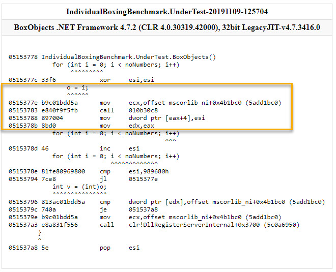
The first instruction (mov ecx, offset mscorlib...) is used to get a reference to the method table of our target type, which also tells how much space must be allocated for each object instance. The 2nd instruction (call 010b30c8) is invoking the function that actually allocates the memory to be used on the heap for the current object instance. The 3rd instruction (mov dword ptr [eax+4],esi) copies the counter value to the memory that has just been allocated earlier. The 4th instruction (mov edx,eax) stores the reference to the boxed object, but that remains largely unused *. That’s it for the boxing itself – the rest of the instructions are simply incrementing and comparing the loop counter.

The function that allocates the memory is worth investigating closer. To simplify, there are 2 ways of allocating memory in .NET: (1) sequential allocation and (2) free-list allocation. The first way simply increases a pointer to the location identifying where the current memory in use “ends”. The second way involves looking through a list of blocks of free space for a suitable one.

Us allocating space for an object at a time falls under small object allocation. The allocation itself is done using an allocation helper. There are 2 allocations helpers that can be used: the first one makes use of sequential allocation. Only if this first one fails to allocate the memory required – eg because the current block within which the allocation pointer is repeatedly “bumped” runs out of space – is the second allocation helper, called JIT_New, invoked.

The first allocation helper will be referred to next as the “fast” path, since its implementation consists of just a few assembly instructions and thus executes very fast. The second allocation helper – JIT_New – is the “slow” path, its implementation involving a rather complicated state machine, and a significantly larger number of assembly instructions.

The catch is that the “fast” path can’t always be used, in which case the CLR has to fail back to the “slow” path. In order to see this in action and understand more, WinDbg is used next to break into the code that does the simple boxing we’re referred to previously. Then we’ll simply be stepping into the assembly code, one assembly line at a time. The goal is to see what the “fast” and respectively “slow” paths of memory allocation involve. In order to catch both within the same “step into” debugging session, we start looking at the code not from when the loop counter is 0, but a value further on (hex 0x7259), when the current block of memory used for allocations is about to run out of space. Before looking at the video, a few things to keep in mind:

• You will see the disassembled instructions for our boxing program in the top left pane. The lower left pane shows the registers that are most interesting for now, while the lower pane shows the memory content at a particular region of memory. This specific address displayed in the Memory window allows us to see both the allocation pointer and the allocation limit, since they’re stored in consecutive locations in memory.
• Ignore names that don’t make sense for now (eg Thread Local Storage), since they’re not critical for getting the main idea across
• Content in the Memory window is shown in little-endian order
• Turn to high quality (HD) when watching the video, otherwise it will be difficult to understand the text
• Text within ‘==’ explains what the current assembly instruction does
• The assembly instruction highlighted in red initially is the point where Main starts executing
• The captions will start on one assembly instruction, but will stay on for a while even after the cursor has moved on to the next line, in order to see the outcome of the instruction that just executed
• The diagram seen to the right only focuses on the memory allocation. Therefore operations such as copying of the values themselves as part of boxing won’t be shown on it
• Objects that are being written to are highlighted in red, while objects being read from in the current operation are highlighted in green 
• A red arrow will show up where the current attempted allocation pointer will be
• The sizes of the segments in the diagram to the right aren’t to scale
• The video is sped up over the lines we aren’t really interested in

You see 4 objects being allocated on the heap: 2 of them right before the current block of memory runs out of space, then 2 more in the new block of memory that’s allocated contiguous to the old one.

Notice how the fast path of allocating memory only takes a few assembly instructions. To be more precise, just 9, including the ret:

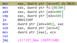
However when the conditions are not right and new memory space cannot be allocated for a new object by simply “bumping” the allocation pointer, the slow path is invoked and the JIT_New allocation helper is called, just like video shows.

Although not immediately visible in the movie above, partly due to speeding up of the video, it takes approximately 750 assembly instructions to execute the JIT_New function, not counting the rep stos instruction that’s doing the memory block zeroing. Giving that the state machine that describes JIT_New is rather complex, it could very well end up taking longer under different circumstances than the ones in the video (eg the next block of memory to be allocated not being contiguous to the previous one, unlike what’s seen in the video; or the need to invoke a garbage collection if the CLR is running out of memory).

We can get an idea about how many times the “slow” path is executed vs the “fast” path, by using a specific type of breakpoint within WinDbg*. Taking several samples by running the same code shows that on average JIT_New is called approximately 15,000 times per all 10 mil objects allocated, the rest of allocations being performed using the “fast” path.

To put this into context, for almost every 700 objects allocated using the “fast” path, only 1 instance gets allocated using the “slow” one. Therefore for our scenario at least, the memory allocation is fast.

The allocation described above represents the first step in the boxing operation – phase (a).

Next in the boxing workflow comes copying the actual data, or phase (b). In our assembly code listing, this is just one mov instruction. 4 bytes are copied from a register to a memory location on the heap. If the “fast” path of allocating memory was deemed fast earlier – itself consisting of a few assembly instructions, then only one mov instruction is even faster.

As for obtaining a reference – phase (c) -, this is happening on its own, sort of speak, since the address of the new object is contained within a register/memory address at the end of each loop iteration. In our example above, it’s the eax register that contains its address.

Therefore phase (a) is fast, phase (b) is even faster, and phase (c) in this case doesn’t take any time. Which makes boxing a rather fast business.

That boxing is not that slow as it’s cranked up to be is even discussed by Jon Skeet’s in this article.

Ok, but if the boxing is that fast, what’s causing our code to be so sluggish? Let’s turn our attention to the ArrayList structure.

ArrayList

We’re coming to the latest stage of our code, where the currently boxed randomly generated number is added to our ArrayList instance.

For navigating the next section, it’s best to skim over the theory part – and just read enough to be prepared for the video below it, which shows a “step into” debugging session into the internals of ArrayList for our whole sample that adds randomly generated numbers to its instance. You can always refer back to this section later on.

The great thing about ArrayList, as well as List<T> and all the types included in the BCL (Base Class Library) is that their source code is available in the Reference Source.

We’re particularly interested for now in arraylist.cs which describes the ArrayList type, and which can be found online here. Of interest to us are:

• The fields belonging to the ArrayList class (lines 45-53):

        private Object[] _items;
        [ContractPublicPropertyName("Count")]
        private int _size;
        private int _version;
        [NonSerialized]
        private Object _syncRoot;
        
        private const int _defaultCapacity = 4;
        private static readonly Object[] emptyArray = EmptyArray<Object>.Value;

• The parameterless constructor (lines 61-66):

        // Constructs a ArrayList. The list is initially empty and has a capacity
        // of zero. Upon adding the first element to the list the capacity is
        // increased to _defaultCapacity, and then increased in multiples of two as required.
        public ArrayList() {
            _items = emptyArray;  
        }

• Add method (lines 199-209), which adds the supplied value at the end of the _items object array and increases the version/size of the ArrayList. This depends on…

        // Adds the given object to the end of this list. The size of the list is
        // increased by one. If required, the capacity of the list is doubled
        // before adding the new element.
        //
        public virtual int Add(Object value) {
            Contract.Ensures(Contract.Result<int>() >= 0);
            if (_size == _items.Length) EnsureCapacity(_size + 1);
            _items[_size] = value;
            _version++;
            return _size++;
        }

• …EnsureCapacity method (lines 341-354), that ensures a large enough capacity value is chosen based on the input parameter. This in turn depends on…

        // Ensures that the capacity of this list is at least the given minimum
        // value. If the currect capacity of the list is less than min, the
        // capacity is increased to twice the current capacity or to min,
        // whichever is larger.
        private void EnsureCapacity(int min) {
            if (_items.Length < min) {
                int newCapacity = _items.Length == 0? _defaultCapacity: _items.Length * 2;
                // Allow the list to grow to maximum possible capacity (~2G elements) before encountering overflow.
                // Note that this check works even when _items.Length overflowed thanks to the (uint) cast
                if ((uint)newCapacity > Array.MaxArrayLength) newCapacity = Array.MaxArrayLength;
                if (newCapacity < min) newCapacity = min;
                Capacity = newCapacity;
            }
        }

• …Setter for the Capacity property (lines 119-129), which when used – and provided the value supplied as capacity is larger than the length of _items – allocates a new large enough internal array and copies across the old elements. Only the “core” of the setter is shown below:

                if (value != _items.Length) {
                    if (value > 0) {
                        Object[] newItems = new Object[value];
                        if (_size > 0) { 
                            Array.Copy(_items, 0, newItems, 0, _size);
                        }
                        _items = newItems;
                    }
                    else {
                        _items = new Object[_defaultCapacity];
                    }

A couple of words about the fields and constants belonging to the type that we’ll keep an eye on. The type of each is within brackets:

• _items (Object[]) represent the actual items being stored in the ArrayList
• _size (int) contain the number of elements currently within the ArrayList
• _version (int), for what we’re interested it simply contains a number that gets incremented with each element addition. Thus it will always be equal in our case with the value within _size
• _syncRoot (Object) – not of interest for us – it’s the 00000000 right before the _size
• _defaultCapacity (const int)
• emptyArray (static readonly Object[]) – contains an empty array (with elements of type Object)

Based on the analysis of the ArrayList inner code and accompanying comments, this is what we’d expect to see happening when running our sample program:

• When the ArrayList is initialised, the internal _items variable will contain a reference to an empty object[] array
• Once the first element is added to the ArrayList, _items will contain a new reference, that points to a new object[] array of length 4 (_defaultCapacity of the _items array). A reference to the boxed int obtained from the first number is placed within this array
• For each subsequent boxed int, a reference to it is placed in the same array
• When the fifth element is added to the ArrayList, again _items will contain a new reference, that points to yet another object[] of double the previous length. This new double array will contain all previously added elements
• The process continues similarly until all the numbers are added

Let’s see next how each number generated gets added to our ArrayList instance, as part of the sample code, and particularly what goes on inside the ArrayList structure as this unfolds. A few things to keep in mind:

• The format is the same as in previous movies: the debugging against the code in Visual Studio happens on the left, while a conceptual diagram showing what goes on gets updated accordingly on the right
• We’ll only look at the first 6 numbers
• You’ll notice a few entries marked as <top>. Those represent type object pointers, which were discussed in the previous blogpost. Their values (hex addresses) weren’t added in order to avoid complicating the diagram. Also – just because <top> was used everywhere doesn’t mean that the address is the same everywhere. In each case it represents a type object pointer, not the type object pointer
• The diagram will not capture the length of the ArrayList itself, which grows by 1 as each number gets added, but focuses only on the internal _items array and its size

Notice how once the internal object[] array gets recreated, the old one no longer matters as no object points to it anymore. The referenced boxed int values remain just as they were, and are referenced by the new array, however the references to them from the old internal object[] array “wither” out in the video, as there’s no longer any practical use for them.

Measuring Up

Based on the fact that the length of the ArrayList‘s internal object[] array doubles once the old one fills up, that we know the target number of elements that are to be added (10 mil), and that we’re starting from an array of length 4, we can easily compute the number of object[] arrays that will be created overall: log2(10 mil) – 1. The value of the logarithm will have to be rounded up, since in the end we’ll need an internal array of a power of 2 large enough to contain our 10 mil elements. As such, this yields 23 internal arrays that get built overall, starting from the default one of length 4, and ending with one of length 16,777,216 (large enough to contain our 10 mil elements). Of course, only one will be “active” at a time, and used to store the ArrayList‘s elements, but nonetheless all of them will take cpu time during the lifetime of our sample code.

Based on the what we’ve seen so far, the following operations are expected to take a non-negligible amount of time:

• (a) Defining all the intermediary internal object[] arrays within the ArrayList instance. This refers to allocating the memory for the respective structures
• (b) Copying the elements from the internal object arrays to the new double ones, when the former are no longer large enough to keep the current number of elements
• (c) Adding one element at a time to the ArrayList‘s internal object[] array. Since we’re looking specifically only at the performance of the inner code involving ArrayList, we’d want to add the same pre-boxed element, as opposed to generating a random number and then boxing it, which were already studied and timed separately before.

An interesting aspect to keep in mind is that ArrayList allows for a constructor to be used that specifies the initial number of elements that can be accomodated. This could have saved time in our sample code by not having to continuously create bigger internal object[] arrays. Yet the List<T> sample operates with the same type of constructor, hence there’s a level playing field.

Given that the 3 operations described above are clear, we can write BDN tests that replicate the activity of each action in the list above as a dedicated method, using only object[]. In order to prevent GCs from occurring, we’ll do 2 things:

• Set the number of BDN operations per iteration to 1, thus allowing only one run of our code to be executed per iteration, followed by the BDN-induced GCs, which clear the slate. This way we don’t allow the memory allocation “effects” to build-up between successive runs, as was the case with the boxing sample previously where 15 operations executed back to back per iteration
• Pre-increase the allocation budgets just enough so in our particular case no GC will occur. The idea behind it is that all the memory allocations we’ll be performing should stay under the allocation budgets, themselves one of the triggers of GCs once exceeded

We’ll create 5 methods, as follows:

• The first method defines an ArrayList instance large enough for our 10 mil elements up front, using a specific constructor
• The 2nd method corresponds to (a) defined previously, and it’s based on ArrayList instances
• The 3rd method corresponds to (b) defined previously, and uses regular object[] arrays
• The 4th method does (a)+(b)+(c), and it’s implemented using regular object arrays
• The 5th method is in terms of workload similar to the previous one, doing (a)+(b)+(c), it’s only that it uses an ArrayList instance

Have a look at the results below (full source code here):

There’s quite a difference between the time it takes to define all the arrays and copying their data as they double (3rd entry) and the time needed for all that plus adding the same reference to the single pre-boxed int (4th entry). One would have expected that the resulting difference to be significantly less than the overall boxing time (30 ms) – after all, in terms of extra work we’re just writing the same exact reference 10 mil times within already pre-allocated object[] arrays, versus boxing which involved allocating memory, initializing it and copying the value to the heap.

The thing is that assigning an element to an object[] is done every single time by calling JIT_Stelem_Ref, a CLR method*. Contrast this to boxing, where allocating memory using the fast path was just a sequence of a few assembly instructions, plus one mov for copying the actual value.

The 5th entry has an even greater time, as the ArrayList implementation is using object[] assignments as well, plus it has some additional metadata to look after (version and size which ArrayList tracks).

Let’s take a quick look at the effective part that adds the same reference 10 mil times to the ArrayList as part of the 5th method above, as it’s converted to assembly code:

Since the loop counter value is stored inside a register, and the time it takes for such a loop based on such a variable to run is ~3 ms, the time for adding the same element 10 mil times to an ArrayList is approximately 114 ms.

Final Assembly Code

As we’ve now looked into each component – and particularly into the assembly code behind them as each was timed in isolation – let’s now make sure that the assembly code for the full ArrayList sample is indeed the sum – and just the sum – of all these components.

We’ll go through each line, including the setup phase before the loop.

==Load the MethodTables's address for the ArrayList type==
0192044f b9fc44285c     mov     ecx, offset mscorlib_ni!DomainNeutralILStubClass.IL_STUB_PInvoke(Microsoft.Win32.SafeHandles.SafeFileHandle,  Int32,  Int32*,  Int32)$##6000000+0x32fa4 (5c2844fc)
==Allocate enough memory for an ArrayList instance==
01920454 e89b2ce1ff     call    017330f4
==Store the address of the recently allocated memory==
01920459 8bf8           mov     edi, eax
==Prepare a register so that it contains the address of the memory we've just allocated for the ArrayList instance==
0192045b 8bcf           mov     ecx, edi
==Call the ArrayList constructor==
0192045d e8267f865a     call    mscorlib_ni!System.Collections.ArrayList..ctor()$##600369A (5c188388)
==Load the MethodTables's address for the Random type==
01920462 b9c05e2c5c     mov     ecx, offset mscorlib_ni!DomainNeutralILStubClass.IL_STUB_PInvoke(Microsoft.Win32.SafeHandles.SafeFileHandle,  Int32,  Int32*,  Int32)$##6000000+0x74968 (5c2c5ec0)
==Allocate enough memory for a Random instance==
01920467 e8882ce1ff     call    017330f4
==Store the address of the recently allocated memory==
0192046c 8bd8           mov     ebx, eax
==Prepare a register so that it contains the address of the memory we've just allocated for the Random instance==
0192046e 8bcb           mov     ecx, ebx
==Prepare another register with the value we're using as parameter in the Random constructor==
01920470 ba01000000     mov     edx, 1
==Call the Random constructor==
01920475 e832ae845a     call    mscorlib_ni!System.Random..ctor(Int32)$##60010F0 (5c16b2ac)
==Set up the loop counter variable==
0192047a 33d2           xor     edx, edx
==The loop counter variable will be stored on the stack==
0192047c 8955f0         mov     dword ptr [ebp-10h], edx
==Load the MethodTables's address for the Object type==
0192047f b9c01b285c     mov     ecx, offset mscorlib_ni!DomainNeutralILStubClass.IL_STUB_PInvoke(Microsoft.Win32.SafeHandles.SafeFileHandle,  Int32,  Int32*,  Int32)$##6000000+0x30668 (5c281bc0)
==Allocate enough memory for an Object instance==
01920484 e86b2ce1ff     call    017330f4
==Store the address of the recently allocated memory==
01920489 8bf0           mov     esi, eax
==Prepare a register so that it contains the address of the Random instance==
0192048b 8bcb           mov     ecx, ebx
==Prepare another register with the value we're using as parameter in the Next method==
0192048d ba0a000000     mov     edx, 0Ah
==Get the address of the Random.Next method==
01920492 8b01           mov     eax, dword ptr [ecx]
01920494 8b4028         mov     eax, dword ptr [eax+28h]
==Call Random.Next (result of the method will be stored in eax)==
01920497 ff501c         call    dword ptr [eax+1Ch]
==Store the recently generated value within the Object instance==
0192049a 894604         mov     dword ptr [esi+4], eax
== Prepare a register with the address of the Object instance==
0192049d 8bd6           mov     edx, esi
==Prepare a register so that it contains the address of the ArrayList instance==
0192049f 8bcf           mov     ecx, edi
==Get the address of the ArrayList.Add method==
019204a1 8b01           mov     eax, dword ptr [ecx]
019204a3 8b402c         mov     eax, dword ptr [eax+2Ch]
==Call the ArrayList.Add method==
019204a6 ff5014         call    dword ptr [eax+14h]
==Increment the loop counter variable==
019204a9 ff45f0         inc     dword ptr [ebp-10h]
==Check if loop is over==
019204ac 817df080969800 cmp     dword ptr [ebp-10h], 989680h
019204b3 7cca           jl      0192047f

If you cross-check this code with all the ones we’ve analyzed before for the components you’ll discover that – except for the exact registers and virtual addresses used – they are mostly* identical. See figures 3, 5, 11, 14 and the listing before figure 6.

Why is it important to have the code of the full sample the same as the sum of all the sub-samples? Because otherwise summing up the times for each component and expecting it to be equal to the time for the full sample would be impossible.

The Results Are In

We’ve seen that adding a value already in the cache (the loop counter) to an ArrayList initialized with a parameterless constructor – just like the one in our sample code – for a number of 10 mil times, not counting the time for the optimized loop (3 ms) takes roughly 114 ms on this hardware platform.

Let’s recap the times we’ve measured so far, as they map to our 4 parts of the sample code:

• Loop (optimized): 3 ms
• Generating all 10 mil random numbers: 127 ms
• Boxing all 10 mil numbers: 30 ms
• Adding an element 10 mil times to an ArrayList: 114 ms

Summing up, we end up with 274 ms – estimated time for performing the effective work of adding 10 mil random numbers to an ArrayList, not including any GC time.

There’s quite a long way from our estimated effective time of 274 ms up to 1,14 s measured for the ArrayList sample in the beginning.

Let’s see what result do we end up with if we go about and subtract the time taken for all the GCs from the time the sample code takes.

The Alternate Way

We’ll be using the same idea we’ve previously applied when we measured the time required for boxing, by employing PerfView to extract the blocking GC time. This round however things are going to be slightly simpler, since each iteration of the sample code takes in excess of one second, and as a result BDN decides to use 1 op/iteration. So we won’t have to divide by the number of ops, as we’ve previously done.

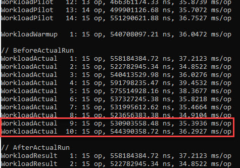
Based on the documentation provided by BDN here (and supported by the numerous runs required for writing this blog post) we need to look at the //BeforeActualRun section of the results, since it’s there where BDN does the actual runs of the operations and measures how long they take. The //AfterActualRun section will contain only those results that weren’t determined to be outliers, adjusted – if the case – such that the overhead time detected is subtracted. The relevant part of the output for our sample code is below:

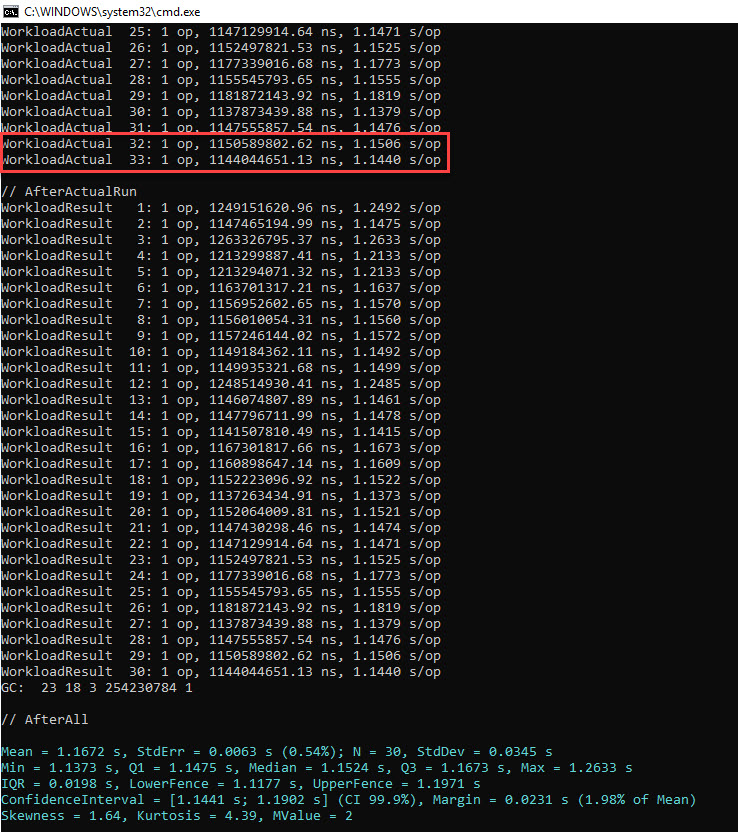
Notice that the 3 of the results were considered outliers and were removed (30 vs 33 results). Let’s look at the last 2 values highlighted, since neither is thrown out as an outlier*, as they show up in both sections referenced before. Let’s identify their corresponding BDN iterations in the PerfView GCStats Excel file, then sum the pause and suspend time; we’ll simply parse the Excel from the end, and keep in mind that after the final iteration there will be only one entry for a induced GC, and after the penultimate iteration there will be only 3 induced GC entries; the rest of the iterations are separated by a group of 4 induced GCs.

That’s a whooping blocking GC time spent of 736 ms out of the total run time of 1,144 ms. It means our code was blocked 67% of the total time it ran by the GC.

GC, Revisited

Unlike in figure 9 in the Boxing section previously, where we only saw “0N” in the “Gen” column, this time we have a lot of values in Figure 16. This is important, so let’s discuss their exact meaning:

• The first digit (0/1/2) is the generation for which the GC ran. Remember that a gen0 GC will collect objects in gen0, a gen1 will collect both objects in gen0 and gen1, and a gen2 will collect objects in all generations including the Large Object Heap (LOH)
• The second digit (N/B/F) is the type of GC that occurred, as following: Non-concurrent GC (blocking GC), Background GC and Foreground GC (this is a Blocking GC of an ephemeral generation that’s triggered during a Background GC only)
• The third letter (I) denotes whether this was a manually-induced GC, that is whether the user’s code actually invoked a GC (using GC.Collect) or the CLR invoked it due to its own reasons (discussed further on)

Why are there so few “0N” entries this time? The fact is that once a GC gets triggered for a particular generation, that gen might not be the final target. As stated by the owner of the .NET Garbage Collector here, once a GC starts, it can actually get escalated to a higher gen. An example: if the conditions for a gen0 GC are met, this will start a gen0 GC, which once running can in turn decide that it will transform to a gen1 or gen2 GC. In fact PerfView’s GCStats contains a dedicated table called “Condemned Reasons for GCs” that lists the initial gen (column 2) and the final one (column 3) – have a look at it below for the iteration displayed previously in figure 16:

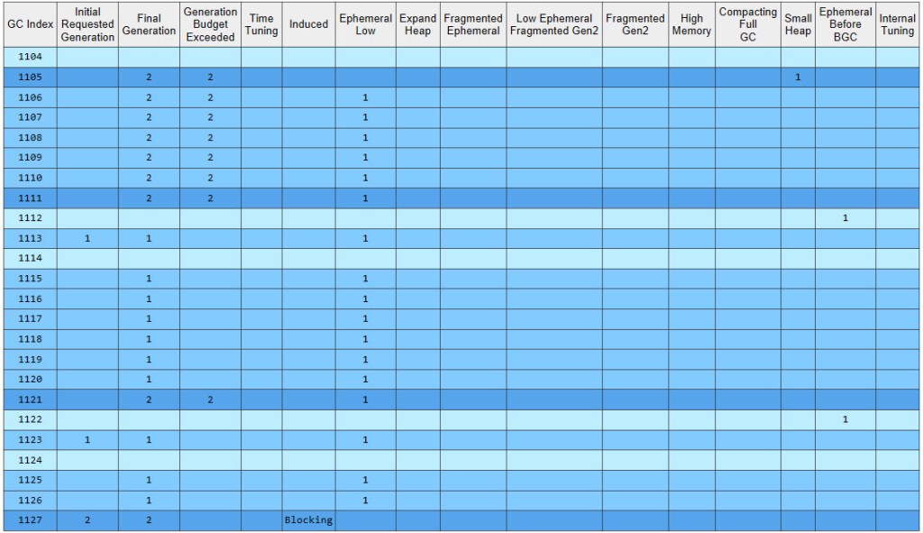
So most GCs just start off as gen0 GCs*, but end up becoming gen1, which is the outcome seen, with the majority of GCs being “1N” in figure 16.

Gen0 and gen1 always share the same segment, called the “ephemeral segment”. From the condemned table we can see that even if the initial requested generation is 0, the “Ephemeral Low” column is almost always flagged – so, unless another reason comes along that justifies raising the final gen even more – then the final generation will be 1*. This is done in order to free up memory in the ephemeral segment, and evicting gen1 objects from it (by either removing the dead ones or promoting the ones that are still live to gen2) is one way of achieving it (Pro. NET Memory Management, Chapter 7, section “Generation to Condemn”).

Another legit question is why the PauseMSec time is several hundred times higher than the values seen in figure 9? The business of the GC is not that simple anymore – it doesn’t just discard all the unreferenced entries in record time like before, but actually has to track a growing number of objects, and then act on them in typical GC fashion (sweep/compact/etc). Unlike in the sample code in the Boxing section, where the boxed ints were no longer referenced by anyone shortly after they were allocated, this time all the boxed objects are kept indefinitely – just as we saw in Video 2. It’s the internal object[] array belonging to the instance of ArrayList that references all these boxed objects. Therefore all the boxed ints will go through generations 0-1-2.

How about the Reason column in figure 16, which gives the reasoning behind triggering each GC? What do these tell? To answer, we need to understand the reasons for which a GC occurs in the first place. Either of the 3 following conditions can trigger it (source here):

1. Allocation exceeds the gen0 threshold or the large object threshold
2. System.GC.Collect is called
3. System is in a low memory situation

The second condition above only happens when BDN invokes the GCs between iterations running our code, so it’s not something we’re interested in. The 3rd condition doesn’t really apply – we’re running in 32-bit mode, eventually allocating ~240 MB (figure 2) out of the 4 GB our process gets (as part of Wow64 mode), yet the OS had plenty of virtual memory to supply (128 TB, subject to RAM + paging file limitation, as described at length here) during all the benchmarks performed for this article.

This leaves us with the first condition as an explanation for all our GCs – allocation exceeding the gen0 threshold or the large object threshold. Which in turn bring us to these reasons (source here; also in “Pro.NET Memory Management, Chapter 7, section “Allocation Trigger”):

• AllocSmall: gen0 threshold has been exceeded
• AllocLarge: large object threshold has been exceeded
• OutOfSpaceSOH: the ephemeral segment is running out of space
• OutOfSpaceLOH: the current LOH segment is running out of space

And in fact, if you refer back to figure 16, you’ll spot AllocSmall as the overwhelming reason for the GCs triggered.

Why so many allocations in the gen0 segment? Because that’s where objects in the Small Object Heap (SOH) get allocated and start their life. And each and every one of our 10 mil boxed int goes there. Neither ever gets discarded, and when triggered GCs analyze them, they’ll be promoted through generations, eventually landing in gen2 and staying there until our code terminates.

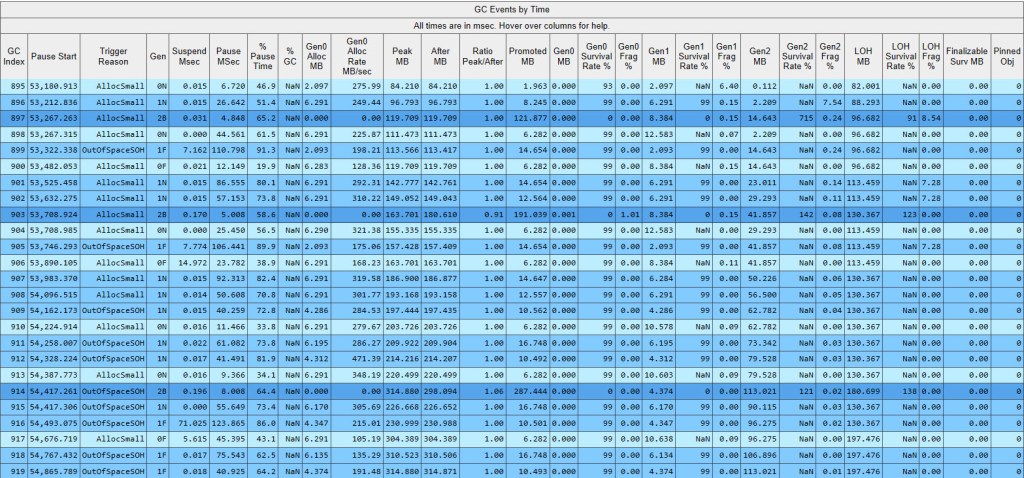
Let’s look at one of the most common kind of GC occurring in this BDN iteration:

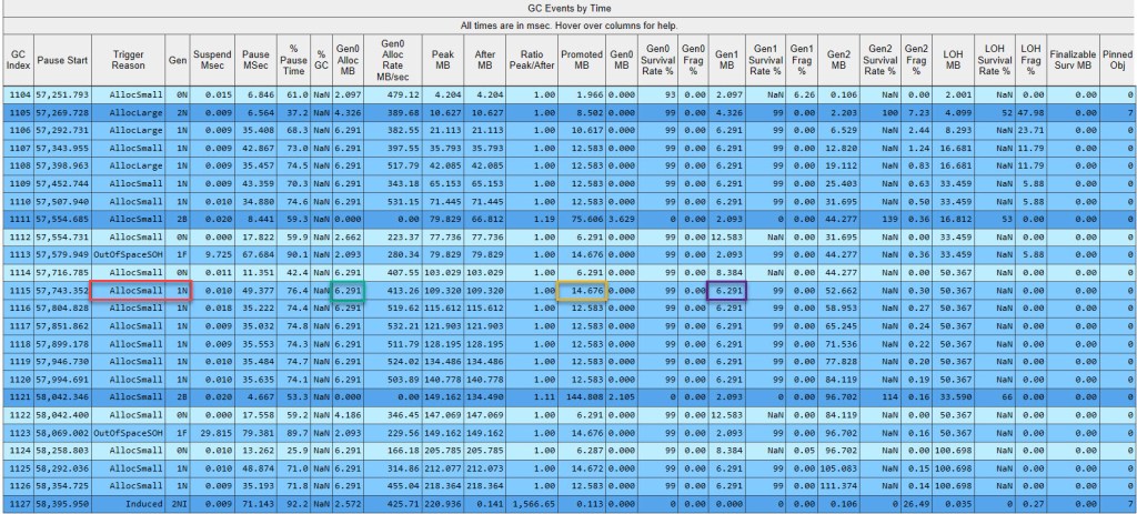
Let’s see what goes on during GC #1115, and how can the various columns be interpreted. The trigger in this case is AllocSmall (red highlight), which as seen earlier means that the allocation budget in gen0 has been exceeded. Why isn’t just a gen0 GC triggered though, but instead a gen1 (red highlight)? If you refer back to figure 17, the only reason marked is Ephemeral Low (1=yes), which as we’ve seen a few paragraphs earlier results in a Final Generation of 1. The Gen0 Alloc MB column (which PerfView’s tooltip indicates as “Amount allocated since the last GC occurred”) contains 6.291 MB, which represent how much the boxed ints that we’ve allocated since the last GC (#1114) consume. Gen0 MB (“Size of gen0 at the end of this GC”) shows exactly 0 bytes, which coupled with the Gen0 Survival Rate % of 99% shows that all the data allocated in gen0 has been promoted by this GC to gen1, whose size is unsurprisingly 6.291 MB (violet highlight – Gen1 MB). Why did everything get promoted? Since our current ArrayList points to all the boxed ints, nothing can be freed up, so a GC will be forced to move the data in the next generation. But being a gen1 GC, #1115 will also go over the data already in gen1 – worth 8.384 MB (Gen1 MB in GC #1114) – and promote it all as well, as Gen1 Survival Rate % shows. The size of gen2 goes up to 52.662 MB: 44.277 MB previously there + 8.384 MB which were just promoted. Nothing else happens to gen2, as #1115 is a gen1 GC and won’t go ahead and process data in gen2 (note the NaN in Gen2 Survival Rate %). How much was promoted overall? 6.291 MB placed in gen1 and 8.384 MB sent to gen2 – overall 14.676 MB (orange highlight).

Summing up the values in the Gen0 Alloc MB column yields the total that ever gets allocated by our ArrayList sample code, which is close to 130 MB*.

There are also 3 GCs that happen due to AllocLarge. This refers to the current Large Object Heap (LOH) allocation threshold exceeded, due to the ever-larger internal object[] arrays belonging to the ArrayList instances allocated there. But why are the boxed ints going to SOH and the object[] arrays to LOH? The rule is simple: objects larger than 85,000 bytes go in the LOH, the rest in SOH. Our object[] arrays – by doubling from an initial size of 4 elements – get fairly quickly over that limit. Each slot of these arrays takes up 4 bytes, the size of a reference on our target x86 platform.

The LOH has its own dedicated segment(s), and it’s sometimes referred to as generation 3. The only type of GC that can process its objects is a gen2 GC.

You can also spot a few “2B” entries in the PerfView GCStats above. As expected, they in turn invoke both a gen0 and gen1 GC, respectively. The PauseMSec values for the 2 background GCs are not that big: 8.441 ms and 4.667 ms, respectively. Remember though that this time they don’t represent how long the GCs took, as was the case when we looked at the exclusive gen0 GCs during the Boxing section, but “the amount of the time that execution in managed code is blocked because the GC needs exclusive use to the heap. For background GCs this is small” (from PerfView’s own tooltip). The background gen2 GC performs the bulk of its work on its own dedicated – GC thread – and that gets tracked separately, as we’ll see a bit later.

The SuspendMSec values are rather high for the gen1 Foreground GCs that occur during the gen2 Background GC. From PerfView’s tooltip for this column: “The time in milliseconds that it took to suspend all threads to start this GC. For background GCs, we pause multiple times, so this value may be higher than for foreground GCs“. But compared to the other column in terms of sums, this is insignificant. And quite important, its values are already factored in the PauseMSec column (detailed explanation here).

Coming back to our computation based on figure 16, the total iteration time of 1,144 ms minus 735.91 ms yields approximately 408 ms.

Let’s do the same subtraction for the penultimate iteration:

1,150.6 ms minus 737.14 ms gives out roughly 413 ms. Similar results.

For both iterations, by subtracting the time spent doing GCs from the overall time, we arrive at results that are roughly 140 ms bigger (~410 ms) than our previous estimate of the actual time our sample code should take on the current hardware platform (274 ms). Of course there’s variance in the times spent between successive runs, but even so, 140 ms is a long time.

Keep in mind that for the 2 iterations whose PerfView GCStats output we’ve seen earlier, one can easily spot 2 gen2 background GCs occurring during each. This will be important next.

Time Thieves

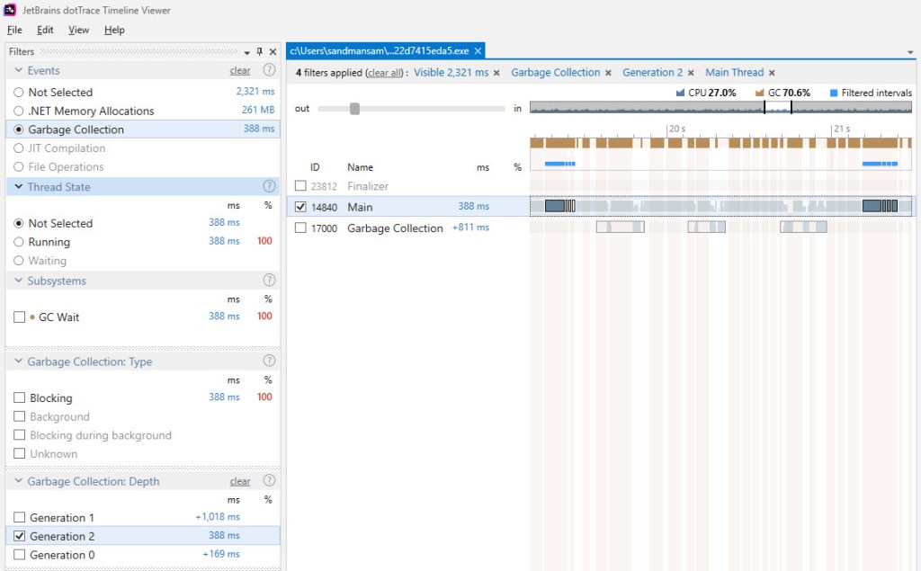
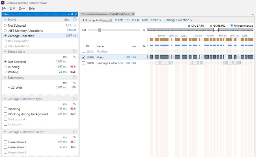
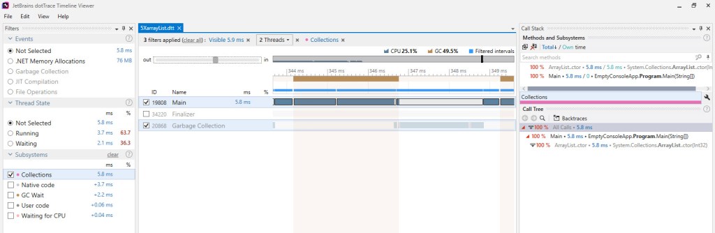
Having admitted that there’s still something going on that we haven’t yet factored in, in regards with the effective time spent in the sample code, let’s look at a close-up during a background gen2 GC, as it occurs during our sample code run by BDN, which now has dotTrace attached:

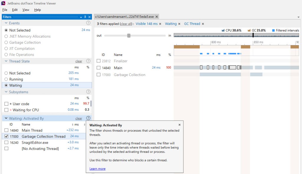
The image above captures one of the gen2 background GCs that occurs during an iteration of the BDN benchmark for our sample code. The highlighted bars represent the time when the Main thread – that’s running our code – had to wait for the GC thread, which runs the gen2 background GC. Notice that most of this time doesn’t fall under “brown” bars – which dotTrace uses to identify either blocking GCs occurring or EE suspensions/resumes. Based on the fact that dotTrace takes its “brown” bars information from the same source as PerfView, namely ETW events, we can safely conclude that this wait time seen in the picture above hasn’t been considered yet in our computations*.

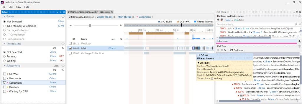
So how much wait time do we have per one iteration? First let’s zoom out and capture the whole iteration in the dotTrace output:

Notice the gen2 GCs on the Main thread, which occur as a result of BDN invoking them after each iteration. It’s easily to distinguish between these and the ones that get invoked as a result of our sample code allocating memory – ours are only of the type background, as PerfView showed; and these occur on the Garbage Collection thread.

There’s one apparent surprise here though: you can see 3x gen2 background GCs occurring, as opposed to 2 we’ve become accustomed so far. Why is this so? dotTrace does bring its own non-negligible overhead – you can actually see that the time spent in this iteration is above 1.5 s (it’s about 1.7 s when measured), quite far from our previous average of ~1.1 s. It’s under these circumstances that most likely the 3rd gen2 background GC occurs*.

It follows though that all the times involved will be skewed – and definitely larger that would be observed without dotTrace running along – so this must be kept in mind. Let’s see how much the Main thread waits on the GC one during this iteration:

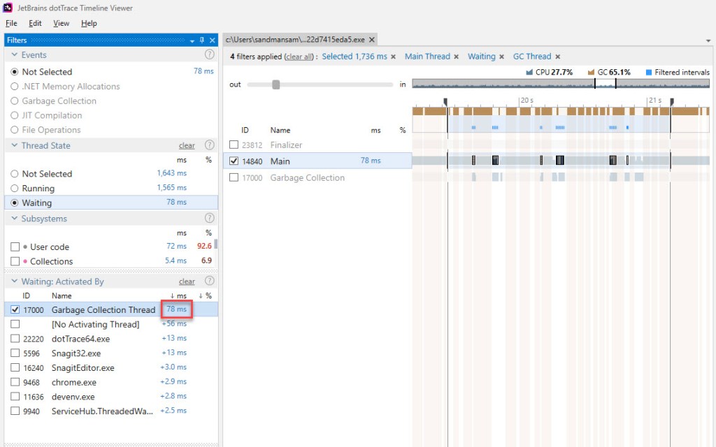
So 78 ms are spent waiting in one iteration of the BDN sample code, but do remember that this includes the overhead mentioned above. Also, some of these wait times occur during blocking GC, which we’ve already subtracted: zooming in and summing yields 26 ms of wait time that fall within blocking time. That leaves 52 ms in pure wait time. When taking dotTrace out of the equation, that time will go down – to something like 30 ms (assuming a similar proportion in regard to the real run time representing 65% of the run time with dotTrace attached – 1141 vs 1736).

That still leaves us with about 100 ms unaccounted for (the difference between the previous few dozen milliseconds up to 140 ms).

What is causing this remaining time then? I don’t have any proof at this time, but I think it’s time that the background GC “steals” from the Main thread. Assuming that the 2 threads run each on a separate cpu core, it’s still the same managed heap that both threads need to access. For example the Mark phase, where each object in the heap is “visited” to determine whether it’s still needed or not – even if we leave inter-thread lock mechanism aside for a moment (which theoretically we accounted for in the “waiting” discussion) there might still be instructions against the heap running on both threads resulting in contention.

To put things into perspective though, the unaccounted 100 milliseconds do come down to about 9% of our sample code time (1.1 s), which is dwarfed by the blocking GC time which consumes most of the time while running the sample code.

Why can’t dotTrace show the real GC percentage at a glance?

We’ve ended up with the following breakdown of time for our complete ArrayList sample is as follows:

• 287 ms effective work
• 775 ms blocking GC / suspending EE
• 100 ms due to contention between GC and the methods doing the actual work

That rounds up to about 25% of the overall time being effective work, with the rest of 75% being the direct or indirect result of GCs occurring, for our ArrayList sample that boxes 10 mil int values.

Like it was said before, there’s quite some overhead introduced by dotTrace, but even so the percentages of how much was spent doing what should stay similar when going from the standalone BDN benchmark to the one “shadowed” by dotTrace.

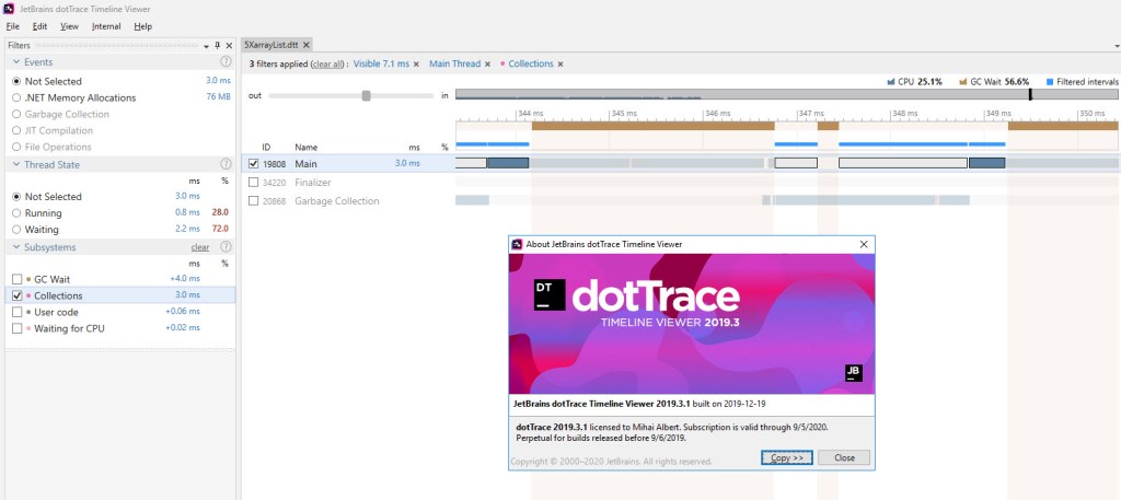
Yet looking at the dotTrace output against one iteration of the BDN code doesn’t make the GC time look that high. Take a look at exactly one such iteration below (Update 2/15/2020: figure 23bis has been added):

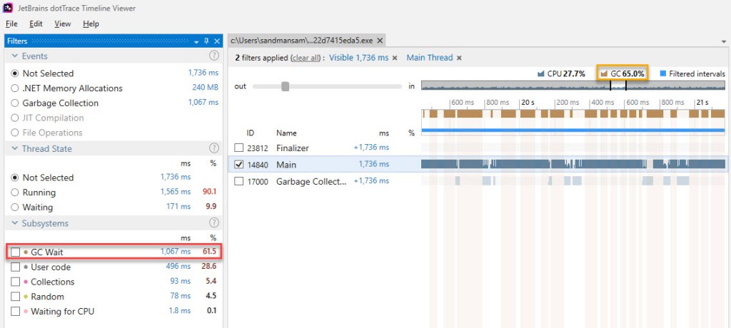
There are 3 things that muddy the waters:

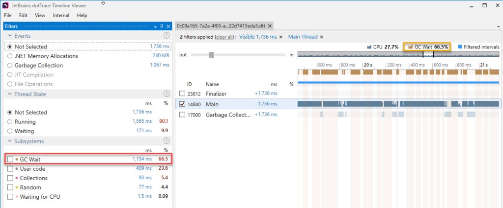
• The numbers referring to GC are rather confusing. There’s the subsystem named “GC Wait” (red highlight on the picture above) and then there’s the “GC” entry on top of the main view (orange highlight). The numbers for these two are slightly different. The documentation explains things, and it basically comes down to the fact that “GC” includes both EE (execution engine) suspensions and blocking GCs, while “GC Wait” only captures the GCs themselves. Also, “GC” refers to what percentage the brown bars (blocking GC) represent out of the visible window (or the current selection within it) regardless of threads, while “GC Wait” aggregates the actual GC time from all the “ticked” threads. If you look at the first picture below, around when the 3rd gen2 GC occurs on the GC thread, one of the brown bars is larger than the segment denoting a GC occurring on the Main thread, which accounts for the difference between the 2 GC values observed previously (61,5% vs 65,0%). Update 2/15/2020: The current version of dotTrace Timeline Viewer (2019.3.2) has rebranded the “GC” label and now shows consistent numbers across the board, as can be seen in figure 23bis above. Note that the same portion of the trace as that in figure 23 is displayed
• Other subsystems show up with more time on the Main thread because the thread itself is waiting or being delayed by activity on the GC thread as a result of a gen2 background GC. We’ve looked at this at length in the previous section
• Other subsystems get to contain the time spent in GC, because some of their methods invoke the GC (eg “Collections” subsystem sometimes “steals” time from the “GC Wait” subsystem, simply because ArrayList‘s Add method occasionally results in a GC being invoked)*. Update 2/15/2020: Ever since version 2019.3, dotTrace Timeline Viewer no longer has this limitation – check the question here.

To sum things up, it’s plainly visible that the GC does take a lot, but not quite as much as it does in reality. The next version of dotTrace (2.3) – scheduled to be released in December 2019 – should address some of these problems. I’ll update the article then (update 2/15/2020: this section has been updated based on the newer version of dotTrace).

To conclude, it’s not that boxing takes long, but that the structures it (quickly) creates in memory determine the GC to spend far more time when it actually needs to analyze and process all that data.

We’ll finish off with some Q&A, and in the next post we’ll look at List<T> and what makes it blazingly fast compared to ArrayList.

Q&A

Q: What would be an example of an operation which in isolation takes little time, but which if not careful gets reported by BDN as taking far longer?
A: We can take the simple example of a function that just defines an ArrayList with a specified capacity. Since the sample code in this post is targeting 10 mil elements, we’ll use this value. Here’s this operation running in a stand-alone sample, and notice that the effective time spent is around 400 us:

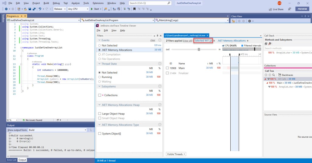
Since that’s all the code does, and then terminates, you see no GC occurring at the end, since that would be pointless (the process’ virtual address space is returned to the OS anyway). Now for a BDN benchmark that does the exact same thing:

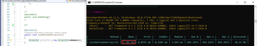
Note that on average there’s less than 1 GC per run, which would make one think there’s no big deal in the time lost to GC, but note the near tenfold increase in the time reported versus our stand-alone sample above. Why? GC’s own time is significantly larger than the operation that just defines the `ArrayList`, and averaging out – against several hundred ops/iteration (since BDN shoots for an iteration time of about 1s looking for consistency) – produces the wrong results. The times can get even greater if the memory allocation budgets are increased ahead of time. For a more complete picture, take a look at this BDN issue I’ve opened here.

Q: Why is the mov edx,eax instruction considered part of the boxing operation? After all, the value is already written in the heap in the previous instruction (mov dword ptr [eax+4],esi).
A: In the sample code used only for timing how much boxing takes, from the perspective of what goes on in the loop only, it’s true that storing the reference to the boxed int (mov edx,eax) is not required, since the value has already been written in the heap, and no one has any need for the reference itself. However right after the loop there’s an unboxing operation – which exists there simply to prevent DCE (dead code elimination) that would have itself wiped out anything in the loop – which needs the reference to the last boxed int. But in terms of operations that boxing consists of, there should be 3: allocate memory, copy the value across, return a reference. Even if storing the reference is not strictly required in this sub-sample, it’s necessary in the full ArrayList sample, and that mov will be there. So besides being in the “theoretical” definition of boxing, the mov helps ensure the full ArrayList sample contains the same instructions as the boxing sub-sample, thus making comparing the run times for each fair.

Q: How can one see how many times a function was invoked using WinDbg?
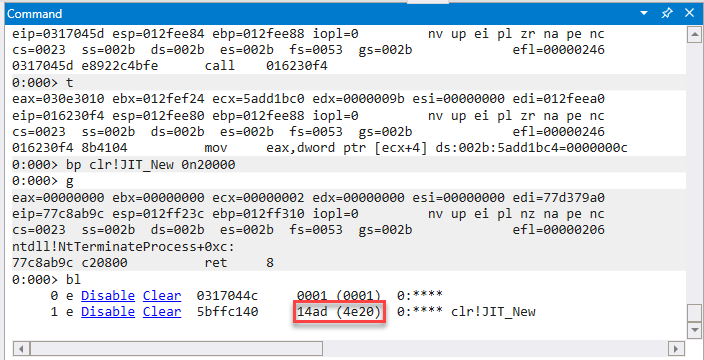
A: Add a breakpoint by running bp <function-name-or-address> 0n<a-high-enough-number>. Once execution continues, every time the address/function is encountered, the value specified initially is decreased. Once execution ends, and provided the counter hasn’t yet reached 0, simply run bl, which will show the value of the number still remaining after all the decrementing. This is actually how the number of invocations for JIT_New was obtained in this article – note the bp command below using the syntax mentioned; WinDbg will decrease the specified counter value by 1 each time the respective address is hit. Since the address is the beginning of the JIT_New function, the net result is that the original counter (chosen to be large enough – 0x4e20 which is 20,000 in decimal) drops to 0x14ad, which converts to 5293. Thus for this particular run, JIT_New was invoked 14,707 times.

Q: How often is JIT_Stelem_ref called when an object[] element is assigned to?
A: It’s called for every single element. Here’s the relevant portion when assigning to the internal object[] array:

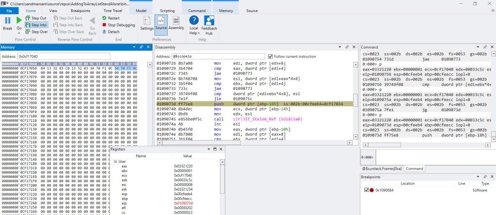
The method that was being executed at the time was DefineObjectArraysEnRouteCopyDataToThemAndFillRestWithSameElement. In the “Memory” window the first 4 bytes (careful to interpret them correctly when grouping, due to little-endian order) represent the type object pointer for object[] array, the next 4 bytes represent the length of the current array (8) and next come 6 references to boxed ints: the first 4 have simply been copied from the static source array, while the last 2 are the same boxed int. The code for the method, including the topmost comment, are here.

Q: I’ve went ahead and looked at the BDN disassembly output for the original sample code here myself. But if I then look at the ArrayList full sample’s assembly code depicted in the section “Final Assembly Code”, it’s not the same thing. Particularly the instantiation of the ArrayList differs, in the sense that the ArrayList constructor doesn’t look to be called in the BDN disassembly (shown below, highlighted in red in top left). It’s the same thing with the assembly code in figure 14. How come?

A: That’s because the code that was analyzed line-by-line actually belongs to a standalone VS project – that contained exactly the same relevant C# instructions as the BDN one – which was profiled using WinDbg. It’s from there that the full sample’s code was extracted and then commented. The difference observed is in the beginning of the code, particularly after the memory for the ArrayList instance is allocated. In the stand-alone sample, the ArrayList constructor is called while for the BDN sample a value mysteriously appears (dword ptr ds:[037916c0]) and a CLR function is called (breaking in the code with WinDbg shows it’s actually JIT_WriteBarrier) instead. Strange as the difference looks at first glance, the outcome of both initialization sequences is the same: the internal empty object[] array gets allocated in memory, then its address is written inside the ArrayList instance in the corresponding field. I’ve actually went ahead and used WinDbg to debug the standalone code, and attach to the BDN one respectively, and verified that in the end they’re both doing the same thing.

Q: In BenchmarkDotNet, what’s the criteria for exclusion of outliers? Eg in figure 15, what’s the criteria upon which the 3 outliers are removed, going from the 33 initial values to 30?
A: As Andrey Akinshin explains here, Tukey’s fences are used. If you want to dive deeper into this topic, it’s worth going through chapter 4 of his book – “Pro .NET Benchmarking”; once you do, the statistics output (turqoise-colored text, following // AfterAll in BDN’s output will become clear.

Q: In the “Time Thieves” section, where the wait state due to BGC is analyzed (figure 20), maybe dotTrace is not marking in brown some regions that PerfView considers to be blocking GC/suspend EE. On this close-up, we’re measuring wait time on the Main thread, which dotTrace is not marking as GC. But what if PerfView actually sees this time as blocking, and included this wait time in its GC time already?
A: There are 2 arguments against that: 1) dotTrace uses ETW, so it relies on the same information as PerfView does in order to render the “brown” bars 2) It’s true that dotTrace is currently missing the 2nd RestartEE events marked as “brown” (but will be visible soon, as stated here), but if you look at the close-up, there are multiple wait events spread across the duration of the GC, which indicate it’s not the RestartEE ones (there’s just one extra pair that’s currently not marked by dotTrace, plus the time it usually takes for the EE to be resumed is small).

Q: Why are there 3 background GCs (BGCs) when dotTrace is run in parallel with the BDN full sample benchmark, as opposed to 2 when dotTrace is not running?
A: I’m not really sure why. You can see below the GCStats tables for the last iteration. You’ll note that there are 25 GCs occurring now instead of 22 as seen when dotTrace wasn’t running and quite a few OutOfSpaceSOH-triggered GCs. It’s not that there’s more memory allocated overall – we’re dealing with the same exact amount. The extra time is not the direct cause – Time Tuning is never marked, so we know it’s not time that triggers the extra GCs (including the extra gen2 GC). I’d dare to say that delay induced by dotTrace running side-by-side affects how often the triggers for a GC are analyzed, which results in a different state that in turn “fires” GCs differently.

Q: I’ve looked at figures 23-25, but neither contains an example of the “Collections” subsystem having time allotted to it due to one its types’ methods invoking a GC.
A: True, on that specific instance there’s no in-your-face occurrence. But consider the example below, which represents a dotTrace capture of a few ArrayList instances being defined, where you can see the Collections subsystem encompassing the blocking GC as well (full context is here):

Notice also that the BGC’s work results in blocking the Main thread, and the wait also gets attributed to the “Collections” subsystem.

Update 2/15/2020: The current version of dotTrace Timeline Viewer (2019.3.1) now correctly excludes blocking GC time from subsystems. The same trace above has been reprocessed using the new version. Notice that the Collections subsystem now excludes the time spent in blocking GC (brown bars on top). Be advised that just opening an older trace with a the new dotTrace Timeline Viewer will not reflect the updates; one must actually reprocess the capture using a custom sequence involving starting the Timeline Viewer from command line – the full procedure is here.

Q: So boxing is taking a value from the stack and placing it on the heap?
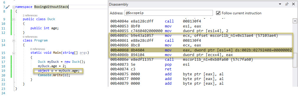
A: Not necessarily. Boxing is converting a value type instance to a reference type instance. There’s no “stack” or “heap” in the definitions used for the term “boxing”. Take the example below (code on the left, resulting assembly code running on the right), whereby a value type instance (myDuck.age) stored as part of a reference type instance (myDuck, of type Duck) on the heap gets converted to a reference type instance (o, of type object). The boxing operation happens in one C# line (highlight on the left), and in 5 assembly code lines to the right (in order: get the address of the method table for type object, allocate memory just enough for one instance, store the address of the memory instance, store the source value to box in a registry, place the value stored in the registry directly on the heap where the new object instance has been allocated). The line highlighted in grey to the right (the currently executing line in WinDbg) holds the key for this scenario: the value type instance is read from the heap and stored in a registry, and the latter is used to copy the value to the heap. No stack involved.

Q: I’m seeing the type fields are not in the order they’re defined in within the ReferenceSource. Eg looking at Video 2 starting at 4:37, in the memory window one can see, in order: ArrayList‘s type object pointer, followed by the address of the internal object[] array, followed by a 0, then followed by _size/_version. Yet in the Reference Source ArrayList direct link, _size follows _items immediately. Why is this so?
A: By default the compiler will place the object instance fields in memory as it best sees fit. As per “CLR via C#”:

To improve performance, the CLR is capable of arranging the fields of a type any way it chooses. For example, the CLR might reorder fields in memory so that object references are grouped together and data fields are properly aligned and packed. However, when you define a type, you can tell the CLR whether it must keep the type’s fields in the same order as the developer specified them or whether it can reorder them as it sees fit. You tell the CLR what to do by applying the `System.Runtime.InteropServices.StructLayoutAttribute` attribute on the class or structure you’re defining.[…]

Jeffrey Richter. CLR via C#

Q: How can I see the calls to and the time inner .NET methods take (eg ArrayList‘s own EnsureCapacity)?
A: dotTrace can be used to obtain this. As described here, I wasn’t very successful in getting Visual Studio to work just as well.

Q: How can one use BenchmarkDotNet?
A: The documentation is pretty straight forward. Start here.

Q: How can one break execution right when the Main method starts in a .NET application, using a debugger?
A: Using WinDbg Preview – which was used in this article – start debugging the executable, then in the command window type sxe ld:clr (to stop when the clr module is loaded), followed by g. Then issue .loadby sos clr (to load the SOS debugging exception). Next add a breakpoint to stop right at Main: !bpmd <exe-file> <class-containing-main>.Main followed by g. For some reason, the last command needs to be run twice, at least with the current version (1.0.1910.03003).

Q: How can the execution be stopped on a specific line in assembly code, provided a specific register contains a specific value?
A: The breakpoint command to be used is bp <address> "j @<register>=<value> '';'gc'". Unselect any addresses copied, otherwise there might be artifacts leftover later in WinDbg, when stepping into/over at that specific address.

Q: In the boxing video (video 1), I’m seeing the rep stos instruction stepped into rather fast, even though it was supposed to run for 8092 times. What’s going on?
A: The rep stos instruction that clears the memory is not stepped into 8 KB times (for obvious reasons), but a breakpoint is set on the next line, that’s why ecx suddenly drops to 0. A concise description of rep stos is here.

Q: In the boxing section, the hex addresses of the various functions/instructions are different between figure 11 and video 1. How come?
A: The various disassembled code / assembly code is captured based off different runs of the same code. Each time the code runs it will usually be loaded at a different address, thus explaining the differences seen.

Q: Once the conceptual diagram “slides” towards the left in the ArrayList sample movie, thus taking the stack away from view, isn’t the o variable supposed to be pointing to every boxed int, as each gets generated? I’m not seeing any arrows coming in from the left, as before the “slide”.
A: On the “Heap (cont.)” part of the diagram the links towards the heap elements from the stack are no longer shown, as to not complicate the diagram needlessly.

Q: The way the conceptual diagram is drawn for the ArrayList sample movie is a bit strange. Sometimes things get painted as they happen in the code, but sometimes not. How come?
A: In some instances, the diagram is painted “by discovery”. Eg at the first boxed number, where the content of the heap cells on the diagram is filled as-you-go while exploring the content of the variables one by one using the memory tab on the left. Sometimes however the diagram is updated right as things unfold, eg for all the numbers except the first one, the diagram is updated right away with the address of the boxed int on the conceptual diagram, despite not showing this anywhere at the time on Visual Studio’s Memory windows. As to why this was done: the end goal was to make as clear as possible the inner mechanisms in a limited amount of time corresponding to adding just the very first elements.

Q: On the conceptual diagram within the ArrayList video 2, the sync block indexes aren’t shown. Why?
A: There’s no added value in representing it for our current discussion, which is why it was omitted.

Q: In the ArrayList movie (video 2), I’m seeing a bunch of memory locations being updated while stepping over/into, aside from the effect of the instruction actually being run. What’s going on?
A: There’s “contamination” due to the debugger. For example at 02:23, you see a couple of times 3 bytes repeatedly written, belonging to the numbers object – a type object pointer, the address of the numbers variable, and a sync block index (set to 0).

Q: How much is the overhead that PerfView brings when collecting under “GC Collect” only?
A: Negligible – just take a look at figure 15 (taken when PerfView was running in the background) and note that the values there match well with the average value in figure 2 (taken with just BDN running).

Q: In the memory allocation video, the size of the object for which we’re allocating memory is obtained from  [ecx+4]. How come?
A: Previously in the video it’s shown that ecx stores the MethodTable’s address. The size of the type whose instance we’re allocating memory for is extracted from within the object’s MethodTable, which is at MethodTable’s address +4, as seen here in figure 9.

Q: Why is the size of the boxed int 12 bytes?
A: On our x86 target architecture, a block of 12 bytes contains – in order: the method table address (4 bytes), the value itself (4 bytes) and space for the sync block index for the next object that follows (4 bytes).

Q: In the output of BDN, once the workload iterations are done, one can see a line like GC: <5 numbers>. What does this represent?
A: In the method output section, BenchmarkDotNet will indicate the number of GC collections per 1000 runs, however in the overall GC stats (GC: <5 numbers>) the number of gen0/1/2 GCs are absolute numbers (not per 1000 runs). Also, in the overall GC stats, the absolute number seen for gen0/1/2 GC runs is the total one observed when running the last <n> operations which make up the last iteration, where <n> is the last number displayed of the 5 numbers after “GC:”. Note that the line in question is officially used for interprocess communication between the host process and the benchmark process spawned for each method benchmark, as described here. Look at figure 15 for an example, and remember that a GC for one generation automatically triggers a GC for all lower generations. In figure 16 you can see that overall there are 23 GCs, out of which PerfView marks 3 as gen2, 15 as gen1 (including the 3x gen2, that gives 18 gen1 GCs), 5 as gen0 (including the 15x gen1 and 3x gen2, that gives 23 gen0 GCs).

Q: What would have happened if a gen budget pre-increase wasn’t done in the ArrayList BDN tests? Why was it so important for this operation to be performed?
A: Here’s how things look like without the budget pre-increase:

You can see that unlike the results in the article, this time there’s GC activity (orange highlight) and in consequence the time for the methods affected grows significantly (red highlight). The 2 methods that originally copied data (seen in figure 13) no longer show up in the results since they had to be removed, as they relied on the defined object array as a source for data copying; but the object array itself had to be removed since it that was how the gen budgets were increased in the first place.

Q: What other way is there aside from [MethodImpl(MethodImplOptions,NoOptimization)] to try and get the JIT to store a variable’s instance within the stack as opposed to a register?
A: volatile can be applied to that variable at the class level.

Q: In the Boxing section, what’s up with the int v = (int)o instruction at the end of the method?
A: It’s there to prevent DCE (dead code elimination). Since we never reuse any of the boxed int values, the compiler is smart enough to simply leave that code out altogether. Having an artificial reference placed at the end prevents this behavior, and gets the boxing code to be generated, thus allowing us to measure it.

Q: In the memory allocation movie, if one looks over the assembly code that does the memory allocation, the lines that were just executed change in WinDbg. Why?
A: It appears that the instructions stepped over don’t actually change, but their opcodes are wrongly interpreted, since the address of the previous instructions are somehow messed up in WinDbg. I’ve opened an issue here.

Q: How can the number of GCs performed during a specific benchmarked method be seen with BenchmarkDotNet (BDN)?
A: Simply decorate the class containing the benchmarked methods with the [MemoryDiagnoser] attribute.

Q: How can the disassembled code for a BDN benchmark be seen?
A: If using Visual Studio, within the “bin\Release” folder you’ll find another folder called “BenchmarkDotNetArtifacts” which contains all the text outputs generated by the benchmarks ran so far, along with a folder called “results”. Within this folder you’ll find the assembly code for the benchmarked methods, under several formats.

Q: How can the number of operations per iteration be controlled within BDN?
A: You can use a specific class for defining the configuration for BDN to use. Take a look at this code snippet.

Q: From Maoni’s blog post here, 3 reasons are also given for GCs ever occurring, but the large object threshold isn’t mentioned – unlike here. Why is there this difference?
A: I don’t know, I can only suspect that either Maoni’s article dates back from a time when things occurred slightly different, or the large object threshold reason was left out by mistake.

Q: Is there any other trigger that could result in a GC, aside from the 3 ones already presented in the article?
A: As per Jeffrey Richter’s “CLR via C#”, there are 2 more, listed below. Although technically the 2nd one doesn’t result in a “true” GC, but merely releases the virtual memory back to the OS.

– The CLR is unloading an AppDomain When an AppDomain unloads, the CLR considers nothing in the AppDomain to be a root, and a garbage collection consisting of all generations is performed. I’ll discuss AppDomains in Chapter 22.
– The CLR is shutting down The CLR shuts down when a process terminates normally (as opposed to an external shutdown via Task Manager, for example). During this shutdown, the CLR considers nothing in the process to be a root; it allows objects a chance to clean up but the CLR does not attempt to compact or free memory because the whole process is terminating, and Windows will reclaim all of the processes’ memory.

Jeffrey Richter, CLR via C#

Q: Why aren’t there any zero values present in any of PerfView’s Condemned Reasons table?
A: They used to be printed in previous versions of PerfView, but as of the current one at the date this article was written, the zero values are no longer displayed – most likely since like this it helps readability. We know the values aren’t somehow missing since the code is quite explicit, and only prints values that are non-zero:

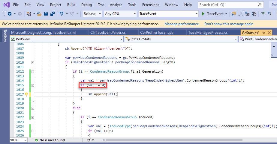
Q: In figure 17, GCs #1106-#1110 have 2 as the final generation (likely because the Generation Budget Exceeded column also points to gen2), but are marked as gen1 (by a medium blue back color, also explicitly in figure 16). Why aren’t these recorded as gen2 GCs?
A: I posted this as a detailed question on Stack Overflow, and upon reaching out to Maoni Stevens – who currently owns the GC component – found out that this behavior is due to a tuning logic that prevents consecutive gen2 GCs from occurring, instead falling back to gen1 GCs. Which is exactly what’s seen in figure 17, whereby #1105 is a gen2 but the subsequent #1106-#1110 get “switched” to gen1 GCs, only allowing #1111 as BGC. There’s work underway to get this backing-away-from-gen2-GCs behavior logged appropriately using ETW, at least for .NET Core, as described here.

Q: Back in figure 18 I’ve summed up the Gen0 Alloc MB column for all the GCs that occur as part of that iteration (minus the last BDN-induced one, of course). Since the ArrayList sample code results in the boxed int values being allocated in gen0, I was expecting the sum for the Gen Alloc MB column to be equal to the size the 10 mil int boxed objects should take, that is 117.187 MB (12 bytes/int x 10 mil objects). But the sum of the column yields 136 MB. Why do I see this difference?
A: The thing is that some of the objects allocated in gen0 never get promoted to gen1. If you look at Gen0 Survival Rate % in figure 18, you’ll spot some of the GCs that collect part of the objects allocated in gen0: #1104, #1111, #1121. They’re easily identifiable by the non-99% value in that respective column. The same thing occurs for gen1 and its survival rate. However if one sums up the size of gen2 after the last GC (111.374 MB at the end of #1126, including the whole gen1 content, since 99% of it was promoted) and the size of gen1 (6.291 MB at the end of #1126, including the whole gen0 content, since 99% of it was promoted) a value quite close to the expected one is found (117.665 MB).What exactly are those objects that don’t get promoted? I don’t know yet, but there’s this request with JetBrains that might help. Once a solution is found I’ll update the article.

Q: Is it possible to have objects on the LOH whose size is smaller than 85000 bytes?
A: Yes, but only if they belong to the CLR. As per Ben Watson’s “Writing High-Performance .NET Code”:

Note. If you go poking around at the objects in the LOH in a debugger, you will notice that not only can the entire heap be smaller than 85,000 bytes in size, but that it can also have objects that are smaller than that size allocated on that heap. These objects are usually allocated by the CLR and you can ignore them.

Ben Watson, “Writing High-Performance .NET Code”

Q: I would like to understand more about how GCs happen in detail, particularly the ETW events generated. Where can I look?
A: Konrad Kokosa’s “Pro .NET Memory Management” is an excellent reference, packed full of details. For example, if you’re after the ETW events and the phases the BGC goes through, refer to figures 11-6 and 11-7 in the book.

Q: In figure 16, 2 background GCs can be seen (#1111 and #1121). They’re in turn supposed to collect both gen0 and gen1 – which happens as well, as both are invoked one after the other for both gen2 BGCs. But why is only the gen1 GC marked as foreground (1F) while the gen0 GC is marked as non-concurrent (0N)? Shouldn’t both be categorized as foreground GCs? As per your post, a foreground GC is “a Blocking GC of an ephemeral generation that’s triggered during a Background GC only“.
A: Good catch ! I don’t have an answer for this, but a question has already been posted on SO.

Q: Some of the BDN benchmarks issue a “The minimum observed iteration time is XXX ms which is very small. It’s recommended to increase it”. Isn’t this bad?
A: A trade-off had to be made between having a large enough iteration time – which BDN achieves by fitting more operations per iteration, thus ending up with a large enough time interval – and avoiding side-effects such as extra GCs that occur due to more than 2 operations stacked “on top of another” as part of the same iteration. The lowest iteration time in this article is seen when defining a single ArrayList, which on the hardware platform tested it takes around a few hundred us. The error seen for that is less than 4% across the 20 individual iterations used. It’s also far away from really quick methods – at and below 1 us, when one would start to be concerned with the resolution of the timers affecting the measurements. Compare this to the increase by one order of magnitude when the GC is accepted in subsequent operations as part of the same iteration under the same scenario, as was described previously, and you’ll find the reason of why 1 op/iteration (unrollFactor=1) was chosen for those. It would be crazy to do the same thing for the benchmarking of the empty for loop, for which one single op is barely observable, but for defining an ArrayList of 10 mil elements that’s not inappropriate at all – considering of course, the hardware platform used. Note also that this approach of 1 op/iteration was only used in the 5-methods benchmark used to time ArrayList operations.

Q: I have the same exact hardware platform as the one used in this article, I’m not running any apps that would consume cpu time, but the times I’m seeing for the benchmarks are pretty different. Eg just defining an ArrayList takes about 200 us during a dotTrace capture, as opposed to 400 us seen previously. What’s generating this difference?
A: The OS version might have something to do with it. Here’s the result for that particular benchmark on a slightly newer version of Windows 10, which was deployed to the very same laptop used to run all the benchmarks in the article:

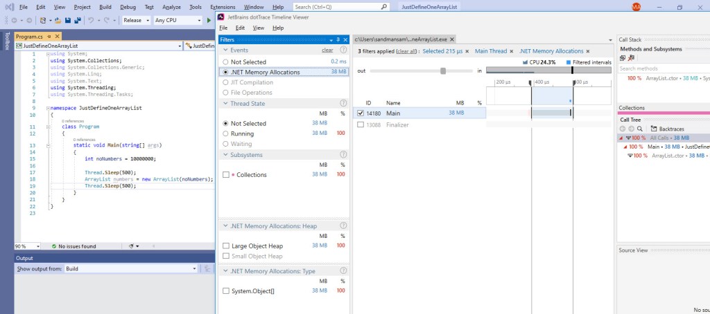
Notice how the times change for the ArrayList benchmarks as well:

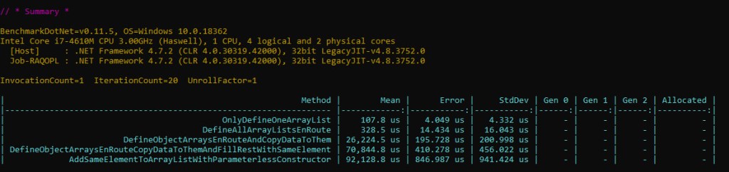
Q: I can’t see the variables’ memory addresses in Visual Studio by using & in front of the variable name while debugging, similar to what’s shown in Video 2 in this article. Why?
A: If the variable itself – as in the address of the instance itself – gets to be stored in a register, you won’t be able to use &. Should that however end up on the stack, it will work just fine. If you’ll look right at the very beginning of Video 2, you can see that the config is “Debug”, thereby ensuring that the stack will be used for storing the addresses of the instances involved. It’s not something specific to the active configuration, as you can very well compile to “Release” but keep [MethodImpl(MethodImplOptions.NoOptimization)] in front of your method, and see that you can use & just fine. Nonetheless, remember that in the end the & operator is illegal for reference types, as was discussed here in the previous blog post.

Q: In this post, there’s a dedicated instruction that does the boxing: object o = currentNumber. But in the first post, there was no such instruction, yet boxing was still occurring as a result of passing an int parameter to a method that accepted object ones. How is each of the 2 type conversions called respectively?
A: They are both implicit type conversions, as no cast operator is used in either version (article here). It’s only that the compiler will create the expected object and perform the boxing itself when it encounters the int value being passed to ArrayList‘s Add method, followed by calling the actual Add method.

Q: What hardware platform was used to run the tests? How about the versions for the software tools/frameworks used?
A: An i7-based laptop was used, whose full details can be seen in the multiple BDN outputs spread within this post. .NET Framework 4.7.2 on Windows 10 x64. As for the tools: BDN v0.11.5, JetBrains dotTrace 2019.2.3, WinDbg (Preview, 1.0.1910.03003), PerfView 2.0.43.